Validation of the interpolation model

The chosen model (in practice the variogram) can be validated by interpolating observed values. If $n$ observations $Y(x_i), i=1,\ldots,n$ are available, the validation process proceeds as follows:

For each $j$, $j=1,\ldots,n$:

• discard point $(x_j, Y(x_j))$;
• estimate the $Y^\ast(x_j)$ by solving the kriging system having set $x_0=x_j$ and using the remaining points $x_i, i\ne j$ for the interpolation;
• evaluate the estimation error $\epsilon_j=Y^\ast_j - Y_j$,

The chosen model can be considered theoretically valid if the error distribution is approximately gaussian with zero mean and unit variance ($N(0,1)$, i.e. satisfies the following:

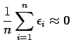
1. there is no bias:
   $$\frac{1}{n}\sum_{i=1}^n \epsilon _i \approx 0$$

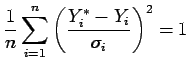
2. the estimation variance $\sigma_i$ is coherent with the error standard deviation:
   $$\frac{1}{n}\sum_{i=1}^n \left( \frac{Y^*_i-Y_i}{\sigma_i} \right)^2 =1$$

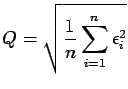
One can also look at the behavior of the interpolation error at each point looking at the mean square error of the vector $\epsilon$:

$$Q = \sqrt{\frac{1}{n} \sum_{i=1}^n \epsilon_i^2}$$

The uncertainties connected to the choice of the theoritcal variogram from the experimental data can be minimized by anaylizing the validation test. In fact, among all the possible variograms $\gamma(h)$, that close to the origin display a slope compatible with the obesrvations and gives rise to a theoretically coherent model, one can choose the variogram with the smallest value of $Q$.