


Next: Kriging with moving neighborhoods
Up: Geostatistics in Hydrology: Kriging
Previous: Validation of the interpolation
Contents
In the validation phase  linear systems of dimension
  need
to be solved. The system matrices are obtained by dropping
one row and one complumn of the complete kriging matrix. This can be
efficiently accomplished by means of intersections of -dimensional
lines with apporpriate coordinate -dimensional planes.
need
to be solved. The system matrices are obtained by dropping
one row and one complumn of the complete kriging matrix. This can be
efficiently accomplished by means of intersections of -dimensional
lines with apporpriate coordinate -dimensional planes.
Note that the krigin matrix  is symmetric, and thus its eigenvalues
 are real. However, since

Tr
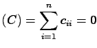
where
Tr is the trace of matrix , it follows that some
of the eigenvalues must be negative and thus is not positive
definite.
For this reason, the solution of the linear systems is usually
obtained by means of direct methods, such as Gaussian elimination
or Choleski decomposition. Full Pivoting is often necessary to maintain
stability of the algorithm.
is the trace of matrix , it follows that some
of the eigenvalues must be negative and thus is not positive
definite.
For this reason, the solution of the linear systems is usually
obtained by means of direct methods, such as Gaussian elimination
or Choleski decomposition. Full Pivoting is often necessary to maintain
stability of the algorithm.
Mario Putti
2003-10-06